About Cell Mapping methods

Cell Mapping (CM) methods are designed for the quick analysis of dynamical systems. These methods discretize the state space into cells and examine the global dynamics.

CM methods are suitable to find

fixed points
periodic orbits
chaotic attractors (usually covered by large periodic cell groups)

CMlib is a C++ library for generating cell mapping solutions, including the following

Simple Cell Mapping (SCM)
Clustered Simple Cell Mapping (C-SCM)
Generalized Cell Mapping (GCM)

The library uses templates in order to allow users to use the data types, differential equation solvers, etc. of their liking.

Documentation

A short guide to CMlib can be found here: cell-mapping-cpp.pdf Doxygen generated documentation can be found here: gyebro.github.io/cell-mapping

Example usage

First you need to include library header

#include "cmlib.h"
#include "pendulum.h"
using namespace cm;

To define your particular system, derive a class from the abstract base class called DynamicalSystemBase. For examples of derived systems see the demo folder. (Note: implementing autonomous systems of differential equations is straightforward, non-autonomous systems can be also implemented by extending the state vector with the time variable.)

Create your system:

double alpha = 1.0;
double delta = 0.2;
double integration_time = 0.1;
Pendulum pendulum(alpha, delta, integration_time);

Depending on the dimension of the state-space, define the centre, width and cell-cound vector for the state space along each dimension. In the following example the system is 2D.

vec2 center = {0.0, 0.0};
vec2 width  = {16.0*M_PI, 10.0};
vector<uint32_t> cells = {1400, 800};

Then execute Simple Cell Mapping:

SCM32<vec2> scm(center, width, cells, &pendulum);
uint32_t max_steps = 20;
scm.solve(max_steps); 
scm.generateImage("pendulum.jpg");

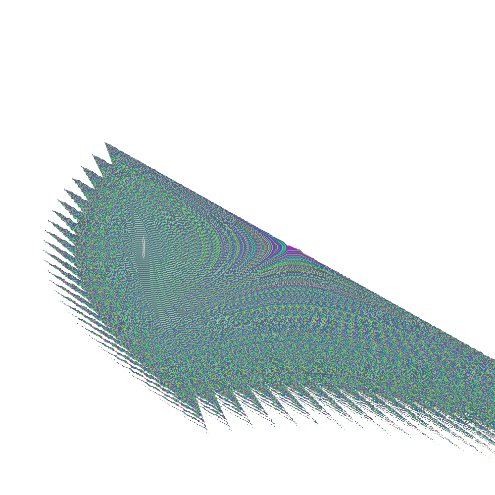
Upon successful execution the resulting output and image will describe objects in the analysed state space region.

$SCM solution of the Pendulum system$

Coloured regions indicate domains of attraction of stable equilibria – fixed points

Clustered SCM example

The ClusteredSCM class can be used to join two (or more) SCM solutions and create a cluster of solutions, which can be extended by additional solutions on demand. This allows continuation of SCM towards state-space regions where trajectories escape to the sink cell, and also makes parallel execution of SCM on separate state-space regions possible.

SCM<ClusterableSCMCell<uint32_t>, uint32_t, vec2> scm1(center, width, cells, &system);
scm1.solve(20);
scm1.generateImage("scm1_initial.jpg");
vec2 center2 = center + vec2({width[0], 0});
SCM<ClusterableSCMCell<uint32_t>, uint32_t, vec2> scm2(center2, width, cells, &system);
scm2.solve(20);
scm2.generateImage("scm2_initial.jpg");

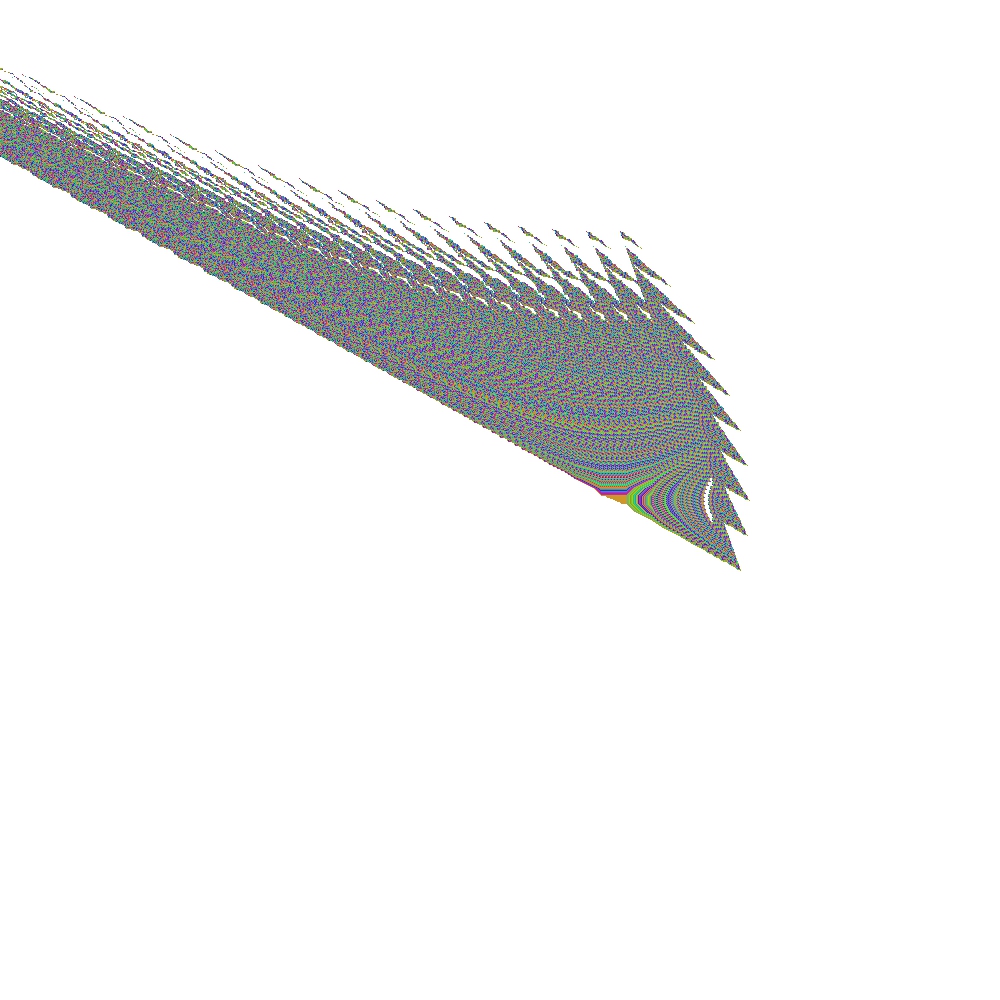
As an example, consider the left SCM solution, which will be extended with a new region (right SCM solution). The following figures show the initial SCM solutions on these two state-space regions:

Joining these solutions can be done with:

ClusteredSCM<ClusterableSCMCell<uint32_t>, uint32_t, vec2> cscm(&scm1, &scm2);
cscm.join(true); // Bool argument controls output image generation

After the procedure is completed, the following outputs can be observed:

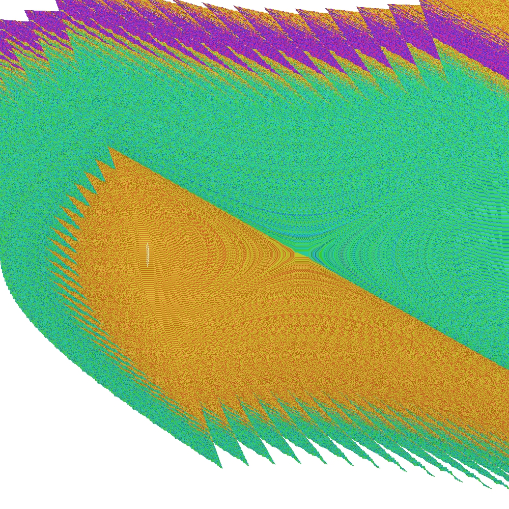
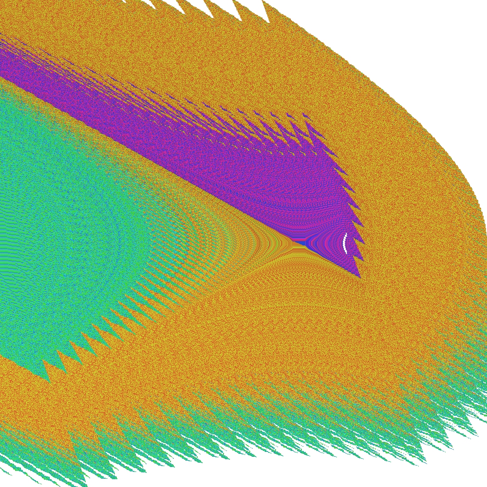
Note, that in this particular example, some periodic groups are at the boundary line between the two state-space regions and they are also discovered by the C-SCM method.